INTRODUCTION
Stone Ridge Technology (SRT) is the proud creator of ECHELON, a leading-edge, high-performance engineering application that simulates fluid flow in the Earth’s subsurface in the presence of injecting and producing wells. Our clients are energy companies seeking to accurately model and forecast the productivity of their global reservoir assets under varying operational, economic, and environmental conditions. Driven by the energy transition, ECHELON can also be used for modeling processes such as the sequestration of greenhouse gasses. It distinguishes itself as the fastest simulator of its type in the industry and the first to be designed from inception for modern GPUs.
Because of its ground-breaking performance, ECHELON is frequently considered a prime alternative when organizations decide to upgrade their simulator software to a High-Performance Computing (HPC) option. Legacy codes struggle to effectively adapt to contemporary hardware, architectural frameworks and algorithms, resulting in significantly inferior performance compared to modern codes like ECHELON. Adopting a new reservoir simulator represents a significant shift for an engineering team, entailing thorough testing, comprehensive analysis, and a rigorous evaluation process. This includes simulating a diverse selection of reservoir models and carefully benchmarking the outcomes, stability, runtime, and costs against an established reference. When considering a transition to a new simulator for production workflows, organizations frequently consider several market alternatives to replace their existing simulator. This blog is intended to help such organizations in setting up objective criteria for such a comparison.
PERFORMING THE EVALUATION
In our experience, evaluations can take one month to one year, depending on the purpose and size of the organization, and they require a substantial effort by skilled reservoir engineers. The best results are obtained when one or more reservoir engineers are assigned the evaluation as a primary task, as opposed to finding time to do it in addition to their normal duties. We will assume in the following, that the new simulator or simulators under evaluation support the same input deck format as the legacy incumbent, either natively or with an automated conversion tool, and specifically there is a single input deck that all simulators under evaluation are capable of reading. This is the most common case and makes the comparison process considerably easier. Even using the same input deck can result in mismatched results because of differences in the choice of default implementations, as we will discuss further on. The evaluation process should be structured to allow for a fair analysis and comparison and provide actionable information. The following are five key activities:
- Choose the models
- Select the simulation hardware
- Understand simulator options and defaults
- Measure key metrics for the comparison
- Factor in the cost
We address these items in more detail below.
CHOOSE THE MODELS
The models chosen for the evaluation should emphasize the organization's principal producing assets but also span a range sufficient to represent features and options present in the company's asset portfolio more broadly. Both black-oil and compositional models, if applicable, should be included in the set, and model size should range from a few 100 thousand cells to 10's of millions or more. The smaller models are useful for assessing the throughput capability of the simulator, a metric that is important when considering ensemble runs. The larger models are useful for assessing overall simulator performance and scalability. Another reason for adding larger models into the evaluation is that the resolution of the present model portfolio may be restricted by the incumbent simulator’s performance limitations, rather than reflecting the resolution a reservoir engineer would like to use for a given study.
Models should be compared in the history match as well as the forecast period. Depending on the organization's portfolio, models with specific features should also be included to achieve broader coverage and stress the simulator with more complex physics such as hysteresis, miscibility, strong capillary pressure, critical point crossing, etc. Forecast models can be tested with a few wells to assess the accuracy of the well model, and with a larger number to test the stability and robustness of field scheduling controls. Models with extreme parameters are also useful in this respect, such as those with strong permeability anisotropy or narrow relative permeability endpoints. Aggressive local grid refinements (LGRs) typically lead to increased numerical heterogeneity and transmissibility anisotropy, as well as high flow throughput, the rate of fluid flowing through a cell divided by its volume. They are therefore a good test for robustness. Other features that might be included if they are in the portfolio are multi-reservoir coupling and/or integration with surface facility networks. If ECHELON or another simulator is missing a major key feature, then it would not be suitable as a total replacement for the organization, but may still provide value on those models it supports. Finally, it should be noted that minor features can always be added by the vendor.
SELECT THE SIMULATION HARDWARE
ECHELON competes with both CPU-based and GPU-capable simulators, and the question of hardware selection for an equitable comparison arises. When comparing a CPU-based simulator against a GPU-based simulator like ECHELON, one should ensure first that the models under consideration will fit on the hardware. This is rarely a problem with CPU codes because memory is typically abundant. Because GPUs use more expensive memory designed for high bandwidth, their capacity is more limited, especially in older GPU models. Simulators also vary in their efficiency of GPU memory usage. For ECHELON, as an example, a million-cell black oil model requires about 3.5GB. A million-cell compositional model requires about N GB to run, where N is the number of components.
Ideally, the organization should test on the same hardware as that which it will deploy, and this should be at or near the leading generation. The state-of-the-art NVIDIA GPU at this time, for example, is the H100. Since it is still in short supply and difficult to acquire, the NVIDIA A100 is the nearest substitute, and most of the major cloud vendors including AWS, Azure, and others offer instances that feature it. The latest version of ECHELON also supports AMD hardware where the state-of-the-art GPU is the MI250 soon to be replaced by the MI300. If it's not possible to access the leading generation hardware, although not optimal, one can test on a trailing generation and scale the results. In general, reservoir simulation performance scales linearly with the memory bandwidth, and one can project performance from older GPUs to more modern GPUs with reasonable accuracy using this technique. Our blog on NVIDIA Hopper also illustrates this point (Leap Ahead with Hopper)
SIMULATOR OPTIONS AND DEFAULTS
Before any meaningful comparison of performance can be obtained, it’s crucial to ensure that all simulators being compared implement the same physics. Differences in the way the flow is modeled can not only affect the results but can lead to dramatically different run times. It’s important to validate that the simulators are generating the same injection, production, and pressure profiles or at least be close, with explainable differences. For simulators that have the same input format and implement the same physical modeling choices (i.e. those compatible with a common legacy simulator), this is often relatively straightforward. However, simulators are very complex software products, and even in this situation, there are often corner cases leading to disagreement. Corner cases refer to situations occurring very seldomly that have not necessarily been treated in academic papers or technical documentation as either ‘not physically interesting’ in the former case, or as ‘being too much detail’ in the second. Below are some examples:
- How should the simulator handle relative permeability endpoint scaling in the limit of coincident endpoints?
- When a combination of rock-fluid models is requested (e.g., hysteresis + miscibility + critical mixing + low salinity), in which order should these be treated ?
- How should fluid properties be extrapolated outside of provided table ranges ?
- How should the gravity-head in a wellbore be computed when the reference depth is far outside the perforation range ?
- If the same operation is requested twice in the same timestep (e.g., a well productivity multiplier), should it be applied once or twice ?
- When should discrete field scheduling actions (such as shutting a well due to economic limit, or automatically opening a well required to maintain potential) be taken ? At the Newton or at the timestep level ? How many actions per timestep should we allow to take?
Due to the complexity of the physical models, simulators implement a series of heuristics to improve nonlinear convergence and stability. Sometimes these heuristics lead to significant differences in results, and it is important to know how to switch them on and off to obtain a fair comparison. Examples:
- Some simulators may damp the well gravity head or the guide-rates by default, while others don’t.
- Different simulators may have different cutoff values for high transmissibility connections, or low pore volumes.
- Some simulators may use different projection schemes in obtaining the grid cell vertical thickness which will impact the well index calculation in highly skewed reservoirs.
It is worth mentioning here that grid editing is very error-prone (in particular for order-dependent edits). It is better to generate grid and grid properties once and reuse them rather than having each simulator generate its own, at least when getting started with the benchmarking process.
If the simulators don’t implement precisely the same physics and heuristics, getting agreement between them is challenging. While this process of discerning implementation differences can be frustrating at times, it can also be very informative. In almost all cases we have observed, the parties involved came to a better understanding of which techniques are actually implemented in each simulator. Furthermore, the process frequently uncovers subtle mistakes in the original model that would be very difficult to spot without another point for comparison.
We would finally like to alert the reader to the importance of technical documentation. It is natural for software vendors to protect their own intellectual property by not revealing key aspects of their solver algorithms or implementation details. Details of the problem solved (i.e., the physical models) and numerical tunings (including convergence and time stepping criteria, exception heuristics, etc.) should, however, be explained crisp and clear, as they impact the quality of the solution and not how we reach it.
Details of the problem solved (i.e., the physical models) and numerical tunings (including convergence and time stepping criteria, exception heuristics, etc.) should, however, be explained crisp and clear, as they impact the quality of the solution and not how we reach it."
MEASURE KEY METRICS FOR COMPARISON
Accuracy
Accuracy is the top concern for evaluation studies. Regardless of speed, cost, or any other metric, a new simulator is not useful if it produces specious solutions and cannot reproduce results from the incumbent. The organization will have volumes of data produced by its current toolset, and it is important to be able to reproduce and re-validate that data as required. Perhaps more than this even, the organization will want to gain confidence in the new simulator by seeing firsthand that it can reproduce the legacy results even when they are wrong or questionable. As an example, a well-known and trusted legacy code does not, by default, have timesteps curtailed by Courant-Friedlich-Lewy conditions including capillary pressure when running in Adaptive Implicit mode. In order for the simulation to run smoothly, a heuristic restriction on the time derivative of the capillary pressure is therefore used. Some modern simulators (including ECHELON) do not need such restriction, and cases with strong capillary pressures may lead to very different water production profiles. In this situation, we find that the client first wants to see that the incumbent results can be matched with the proper setting, before being convinced that the new solution is preferable.
To start the comparison process, one should first assess the fluids in place and make sure there is agreement with the reference. One should next compare field-level quantities, such as pressure, cumulative production and injection, and field-level rates. For gross features such as these, one can expect a close alignment of results, with differences mostly indiscernible by eye. At the next level, one can compare well-by-well production rates and cumulatives where the tolerance may be relaxed. Note that well rate matches usually require validation ‘by eye’ and are not easily automated. Further still, one can compare reservoir properties such as pressure and saturation as the simulation evolves. There are numerous post-processing tools including our own SimDiscover which may be used to do a cell-by-cell comparison of two different simulator runs on the same model. Significant deviations warrant further investigation.
Stability
By stability, we mean the characteristic of being able to perform deterministic runs on the same hardware configuration, and deviations remaining well below physical or modeling uncertainties for different configurations. The first requirement is obvious, and the first test we recommend is simply running the model multiple times on the same hardware. Results should be bit-for-bit identical. Any deviation whatsoever is an example of non-determinism and indicates a problem. Satisfied that the simulator is deterministic, the evaluation should run each model on multiple hardware configurations. For CPU simulators, vary the number of cores and for GPUs vary the number of GPUs. Further, if a simulator supports CPU and GPU, both should be run and compared.
One may wonder why running on a different hardware configuration (e.g., 16 vs. 32 CPU cores, or 1 vs. 2 GPUs) on the same problem would change the solution at all. With all but the most trivial preconditioners, the result will depend slightly on the ordering of the rows of the matrix. Domain decomposition reorders these rows to minimize communication and optimize convergence. Changing the number of domains, therefore, changes the global ordering, and hence, the solution to the linear system every so slightly. Minor differences at each timestep can accumulate in time. Therefore, it is crucial to ensure the system is solved to a specified tolerance. As the tolerance is tightened, the difference in solutions seen with different hardware configurations shrinks. If the tolerance is tight enough, the differences will be well within required engineering precision and perhaps even imperceptible.
Ideally, changes in hardware configuration should yield errors well below any of the other uncertainties present in the simulator data and model. For example, if a user is simulating a model to optimize the location of an infill well which is supposed to increase reserves by 1Mbbl, but running on 16 vs. 32 cores yields a difference in the recovery of 0.5Mbbl across the field, then the simulator errors render this analysis useless. If both incumbent and challenger fail this test in the forecast, then either the model chosen may lack forward stability and thus is not suitable for testing, or convergence criteria should be tightened.
Forward stability is an important concern. Whether executing the simulator on different hardware configurations, using different levels of parallelism or stopping and restarting the simulation at varying times, one should expect to obtain similar results. One caveat is the following: The reservoir simulator’s field scheduling or well scheduling module changes the course of the simulation in discrete ways, e.g. closing a well when the water cut is too high, or drilling a new injector well when there is a perceived injection shortfall. These discrete decisions suffer from the limited precision of floating point arithmetic. Unless special provisions are made in the code, a well that is supposed to shut in at a water cut of 98% will stay open at 97.99999% and close at 98.00001%. That sensitivity can have a disruptive impact when executing the code on different hardware or changing the level of parallelism where floating point and order of operations differences could throw the simulator into different well management regimes. We can identify those highly sensitive models by executing them in different configurations on the reference simulator. If they are not forward stable on the reference simulator, they should be excluded from the selected models.
Solver quality
Improved speed is often the reason that an organization is seeking a new simulator. Advances in recent years with multi-core chips and GPUs have led to true HPC reservoir simulators that offer performance that is significantly greater than that to which the industry has become accustomed with legacy products.
Most if not all commercial reservoir simulators use the Newton-Raphson solution method wherein the equations for a timestep are linearized and solved iteratively (Newton iterations) up to convergence before moving to the next timestep. Each timestep is therefore divided into Newton iterations, themselves divided into linear iterations. What ultimately matters is the performance in terms of elapsed time per physical simulation time (for example, how many minutes does my simulator take to advance one year). How this time is spent in Newton and linear iterations is nevertheless important to judge the robustness of a simulator.
The first thing to compare is a cumulative plot of Newton iterations vs. elapsed time. These plots should, in principle, be similar across simulators or at least have a similar trend, where the number of iterations per timestep would increase around challenging periods of the simulation (e.g., at gas-injection startup, when miscibility kicks in, or with flow reversal in the presence of hysteresis) and decrease during easier periods. Spurious spikes should be investigated and could indicate inappropriate internal heuristics for the problem at hand, or indicate that convergence criteria need to be relaxed. Most importantly, if a simulator shows a much lower number of Newton iterations than another, it is possible that convergence criteria are different, which needs to be ascertained for a fair performance comparison.
The second thing to look at is a cross-plot of Newton iterations vs. linear iterations, which is an indication of the number of linears required to solve a system of equations. Here, only the trend is relevant, i.e., we want to see if the linear solver struggles at certain points in the simulation. Comparing the absolute number of linear iterations is not useful unless we are sure that the same linear solution strategy is used. For example, the current state of the art linear solvers use a multi-stage preconditioner where the pressure equation is decoupled and solved with an algebraic multi-grid method. This significantly reduces the number of linear iterations, but each iteration is more expensive.
It is also important to consider that simulators typically have heuristics to limit the size of time steps to avoid excessive time-integration error. Often, looser tolerances can allow significantly faster simulation, but at the expense of accuracy and reliability. Less often (but we have experienced this), loose tolerances can increase runtime because of unphysical timesteps being accepted, driving the simulator in the wrong direction. Loose tolerances can also lead to difficulty reproducing the same results on different numbers of processes, hardware, or simulator versions. Clearly, having, for example, reserve estimates dependent on these nonphysical parameters is unacceptable.
The above discussion highlights how essential it is to have a clear understanding of the methods and numerical tolerances that are used to assess convergence. For this reason, and the reproducibility issues described above, ECHELON implements the same conservative, industry-standard default convergence criteria as a leading legacy simulator. Furthermore, these tolerances are fully within the user’s control, if tighter criteria are warranted or if looser criteria may be desired for preliminary screening, for example. Only after equivalent convergence has been established can a meaningful comparison of the performance of two simulators begin.
It is also important to consider that simulators typically have heuristics to limit the size of time steps to avoid excessive time-integration error. Often, looser tolerances can allow significantly faster simulation, but at the expense of accuracy and reliability."
Speed and Scalability
When talking about speed and performance, we distinguish between throughput performance and peak performance. Throughput performance relates to the number of models a user can simulate with fixed hardware in a given time. This is particularly relevant in ensemble simulations. For this kind of test, we recommend a model of medium to small size, preferably less than 1 million active cells. One approach to conduct the test is to perform numerous simultaneous simulations on the same hardware, whether CPU or GPU, with the number of simulations designed to saturate but not overload the node or exceed its memory capacity. For instance, a CPU simulator executing on a machine with 2 processors, each with 16 cores, could be used to simulate a single model using all 32 cores, or two models using 16 cores each, and 4 models using 8 cores each to find the best result. For a GPU simulator, we recommend the user execute as many copies of the model as fit on a single GPU without exceeding memory limits. The results achieved are then presented as models completed per second or active cell-years per second if we multiply with the number of active cells per model and the number of simulation years. ECHELON makes it very easy to perform multiple simultaneous simulations on a single GPU using the NVIDIA MPS process. (See Improving GPU Throughput of Reservoir Simulations using NVIDIA MPS & MIG R. Gandham et.al). AMD hardware natively supports multiple running processes on a single GPU as well.
Peak performance relates to the fastest time in which the simulation of a given model can be completed. For this test, we recommend using a large model, preferably larger than 10 million active cells. When testing a CPU based simulator, we suggest parallelizing the simulation using an increasing number of cores until performance peaks. For example, a good procedure is to run on 32, 64, 128, 256 etc. cores until the performance peaks or adding additional cores returns diminishing results. For a GPU simulator, one would follow the same procedure, using 1, 2, 4, or 8 GPUs. One of the great advantages of a GPU-based simulator is the small, compact hardware footprint required. We typically find ECHELON’s performance on a single modern GPU to match that of a modern CPU simulator using 256 cores. Access to 256 cores usually requires 4 nodes, each with two 32-core processors. In contrast, one can easily fit 4 GPUs in a modern node and thus require just ¼ of the node for this comparison. Modern simulators divide large models up into domains which are distributed over computing elements operating in parallel to achieve higher performance. On CPU those domains are relatively small and are distributed over hundreds or even thousands of cores. On GPU the domains are comparatively large and distributed over a few GPUs. For example, if one GPU is the equivalent of 256 CPU cores in performance a model split over just 2 GPUs with a single inter-domain boundary requires 512 CPU cores with boundaries between each of them. Since the domains are so much smaller on CPU, there is less work to do and the ratio of computation to communication is less favorable and thus less efficient. This is another big advantage in favor of a GPU-based simulator.
ECHELON implements the same conservative, industry-standard default convergence criteria as a leading legacy simulator."
Memory usage is another useful metric of simulator efficiency and performance and is particularly important on GPU. Inefficient use of memory means that fewer models fit on a single GPU, limiting throughput speed, and also incurring unnecessary performance penalties with the slosh of additional data back and forth between GPU and CPU. Available GPU memory has grown rapidly over the past decade. The modern NVIDIA H100 packs 96GB where the first Tesla’s offered just 6GB. Efficient use of this resource allows one to run ensembles on a very compact system. ECHELON has been designed to be frugal with memory and supports black-oil models up to 12 million cells on a single 40GB NVIDIA Ampere A100 GPU and up to 27 million cells on the newer 96GB NVIDIA Hopper H100 GPU. By running variously sized models, black-oil and compositional, one can get a measure of the memory required ‘per-component’ and ‘per-cell’. ECHELON scales linearly with both, another advantage when it comes to large and complex models.
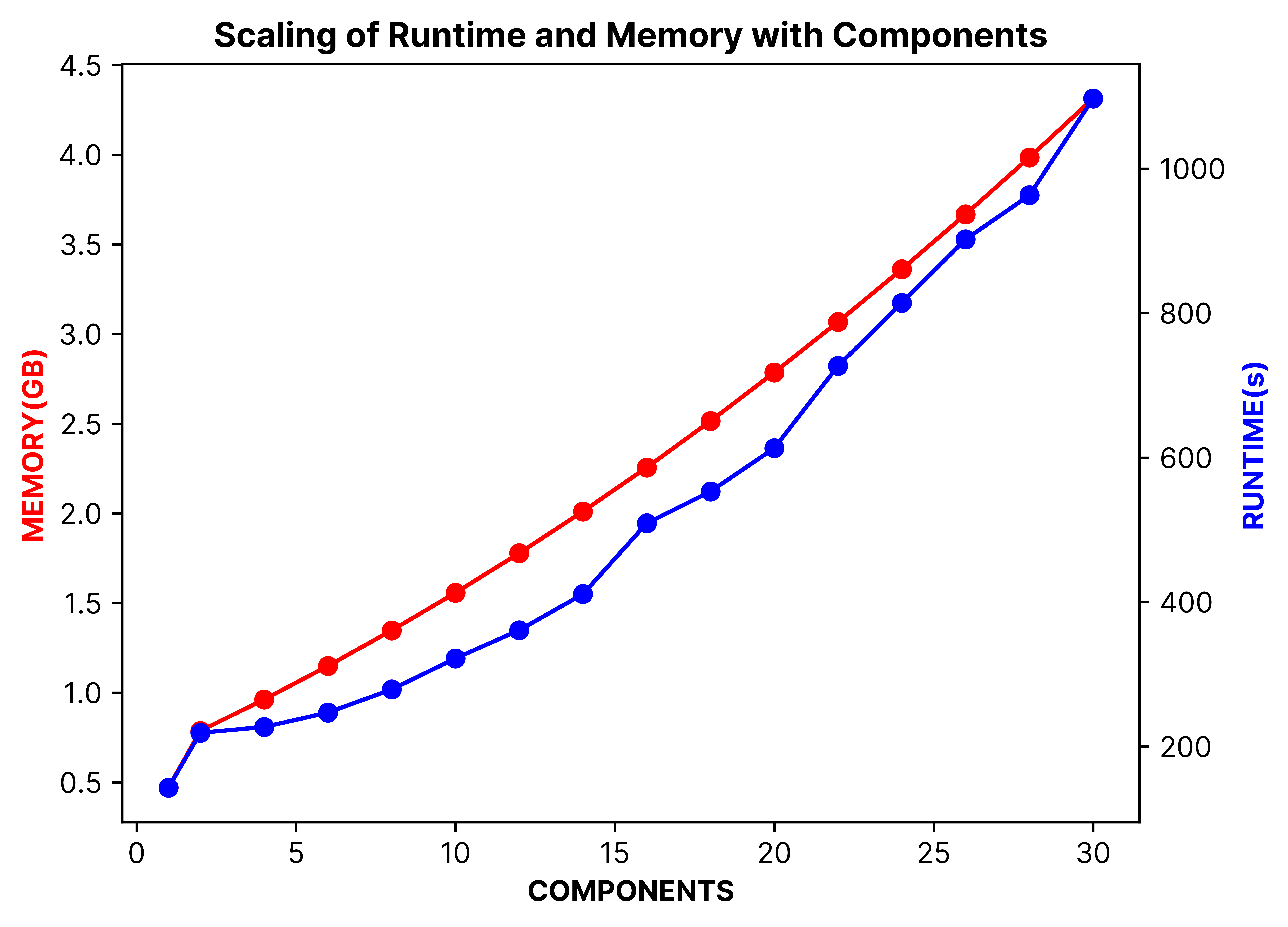
Test Model 1, fully implicit runs. Scaling of the simulator runtime and required on-chip memory as a function of the number of hydrocarbon components, normalized to the figures of the equivalent black-oil model (using a single V100 GPU with 4 CPU threads for the wells). Quadratic trend lines are also shown. From "A Graphics Processing Unit–Based, Industrial Grade Compositional Reservoir Simulator", February 16, 2022, SPE J. 27 (01): 597–612, K. Esler et.al
Other concerns that may influence the timing results include file I/O, queuing system defaults, and OS choice. Evaluations can produce large amounts of data. A slow disk I/O subsystem, a nearly full filesystem, or competing applications running simultaneously and writing to the same disk space can slow the simulation unnecessarily and render comparisons of actual turnaround time inaccurate. Queuing system defaults may influence the number of CPU cores assigned to a process. In some pathological cases, the system may only assign a single core to the run, slowing down the whole process enormously. Even GPU simulators need CPU cores for I/O and other serial tasks. Finally, the OS may have a small impact. ECHELON may run about 10-20% slower in Windows than in Linux, depending on Windows driver settings.
Since the domains are so much smaller on CPU, there is less work to do and the ratio of computation to communication is less favorable and thus less efficient. This is another big advantage in favor of a GPU-based simulator."
FACTORING IN THE COST
Cost is always a factor in the decision to adopt a new simulator. Assuming accuracy and stability are excellent and speed is compelling, cost can be a deciding factor. Cost has components for the software licensing, which usually dominates, and for new hardware if required. When we first started marketing ECHELON in 2016, GPU computing was still a nascent trend, and although impressed with the huge performance boost, many clients did not have access to GPU hardware. Today the situation is reversed, and most new cluster and hardware purchases include GPU capability as organizations have seen the value provided for both traditional compute loads in seismic and reservoir simulation but also emerging compute demand from AI. One approach to comparing simulators using a quantitative cost metric, focuses on the throughput results collected in the speed tests, by calculating the (cost for the required hardware) / ((number of active cells per model x simulation years) x (models processed per unit time)). This measures the cost for a unit of throughput, i.e. dollars per cell-years per second. Other costs to consider would be training and migration costs if, for example, the organization moves to a simulator that requires a different input format than the incumbent, as well as the costs of changing the workflow tools, both those commercial and those developed in-house, that accompany the simulator if such a change is adopted. These quantitative metrics tend to ignore the business impact. For example, the ability to run larger ensembles or to easily simulate fine-scale models with tens of millions of cells may be invaluable and compensate for the cost associated with upgrading the hardware. From the individual engineer’s perspective, the ability to run multiple simulations in a single day, rather than wait days or weeks for a result, greatly improves efficiency.
CONCLUSIONS
Evaluating and comparing competing numerical reservoir simulators takes time and effort. There are numerous considerations that we have highlighted here, starting with the testing model portfolio and including hardware selection, simulator defaults, attention to convergence criteria, accuracy, stability, performance, and cost. When completed, the customer should have confidence in the benefits, quality, and cost of the new product. We sincerely hope that this short blog article was interesting for the reader and that it may provide some guidelines for future testing and evaluation of either our products or those of our worthy competitors.