Physics Informed and Neural Operator Networks

Introduction

Recently, physics informed neural networks and neural operator networks have generated renewed interest in data-driven solution methodologies for physical problems governed by coupled (partial) differential equations. These equations are at the core of most scientific and engineering software applications, including those used for subsurface flow simulations. Consequently, the reservoir engineering community has become attentive to these developments. Strictly speaking, neither approach is fundamentally new, but the emergence of GPUs with hundreds of tensor cores (NVIDIA) or accelerated cores (AMD) and the availability of powerful libraries for neural computing (TensorFlow, PyTorch, etc.) have been the drivers behind current developments. While at the present stage neural networks cannot replace classic full physics reservoir simulators in complex forecasting scenarios or history-matching tasks (we will explain why), there is always the possibility for a breakthrough in the near future, similar to what has happened in the area of generative AI. We think that the topic is important, and we write this blog to give a brief overview that compromises between a detailed technical treatment and the broad scope of the subject matter. We will close by discussing potential applications in reservoir engineering. Due to the complexity of the subject, this blog will be longer than our usual entries, however we hope the additional content benefits our readers.

Neurons and Neural Networks

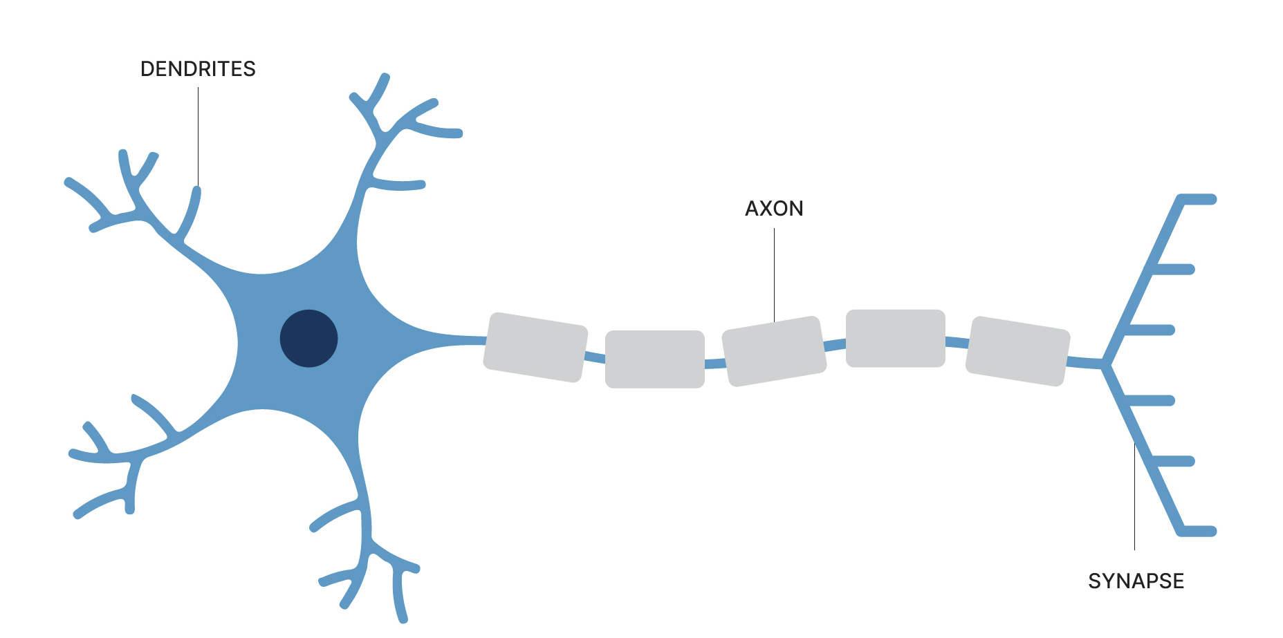
Neural networks are modeled after the animal central nervous system whose nerve cells (neurons) are among the most versatile of cell types, their structure, and function strongly dependent on the specific task the cell has to perform. Examples of biological nerve cells are motor neurons, sensory neurons, and interneurons (See Figure 1). Fundamentally, neurons communicate with other neurons or cells by sending an electrical signal down the axons to their synaptic terminals, where neurotransmitters are released into the synaptic cleft, diffusing and binding with receptor sites on the postsynaptic ending to influence the electrical response in the connected cell. Compared to the complex nonlinear and time-dependent behavior of real neurons, their digital twins use quite a few simplifications and restrictions, specifically:

• Digital neurons inside simulated neural nets do not model any of the dynamic behavior we observe in nature. Input signals don't travel along paths arriving at different times, the signals don't fade, and output signals don't diffuse.
• Digital neuron input signals are held constant until we recompute the state of the network or present a new input to the network as a whole.
• Digital neuron states are held constant until recomputed.
• Digital neuron states are a function of input and bias only.

In summary, computing the state of a simulated network of digital neurons is a process involving discrete steps during which neuron output states are computed as a function of weighted inputs and a bias.

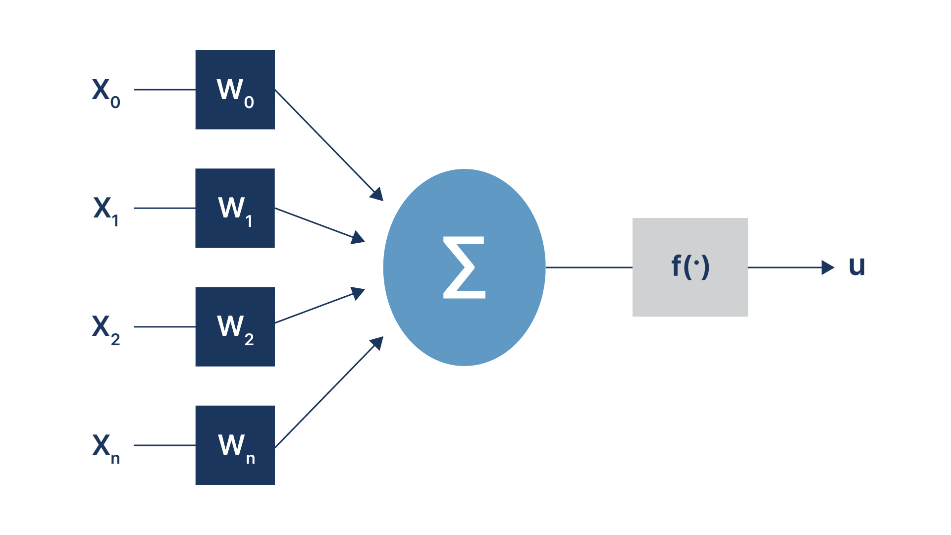
The digital neuron shown in the schematic of Figure 2 is derived from the McCulloch and Pitts neuron described in their paper 'A Logical Calculus of the Ideas Immanent in Nervous Activity' in 1943. Slightly enhanced (use of weights, added bias term, and more flexible output function), it is representative of the neurons used in today's modern deep learning networks. Hence, the fundamental unit of computation has not changed much despite the dramatic progress in the way we construct and train new network architectures. The state of a neuron is defined by an activation function f(.), which takes as its input a weighted sum of the inputs and a bias. The non-linear function f(.) is often a sigmoid function, a hyperbolic tangent, or a rectified linear unit (RELU). In what follows, we will simply refer to digital neurons as neurons.

From Single Neurons to Multi Layer Perceptrons

Although the name perceptron was initially used to denote a single neuron, it soon became the synonym for a layer with two or more neurons used in classification tasks. Pioneering research was done by Frank Rosenblatt, a scientist at Cornell Aeronautical Laboratory, who simulated single-layer perceptrons on digital IBM computers as early as 1958. However, shortly after its inception, researchers became aware of a fundamental limitation of the architecture.

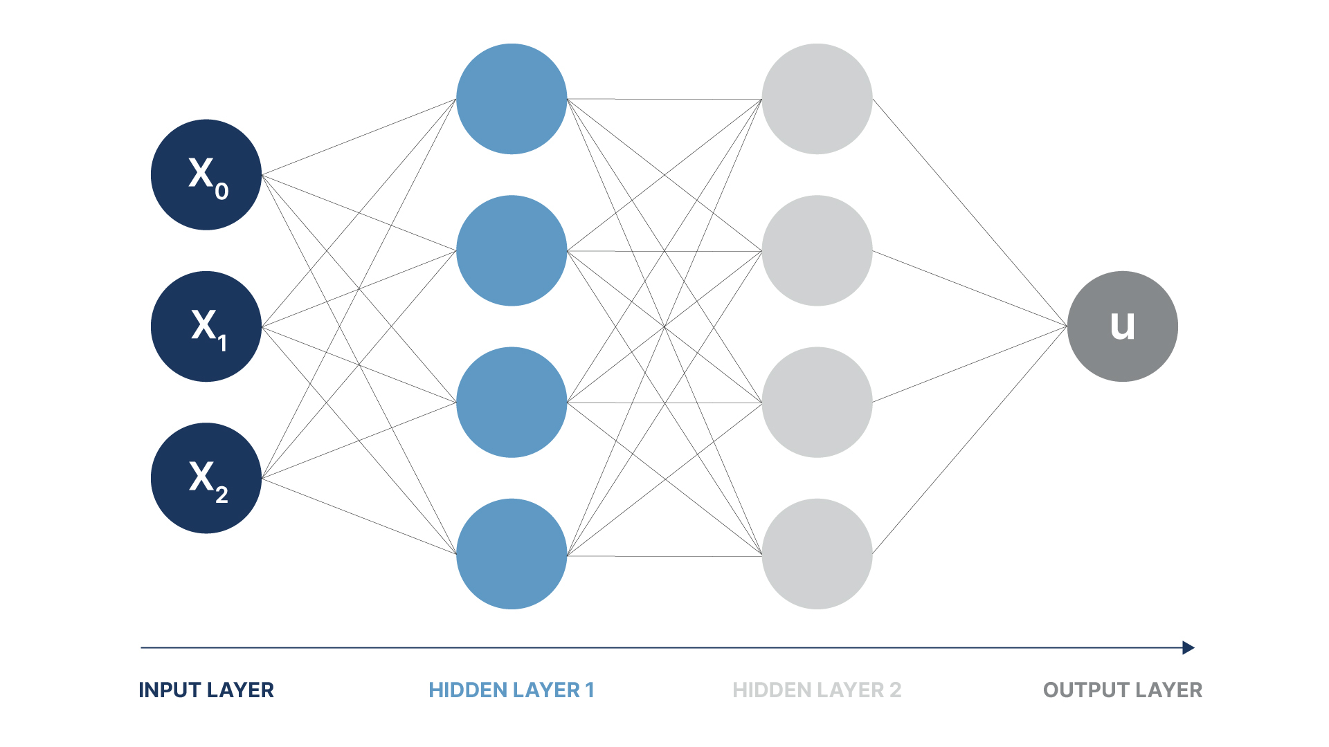
It turned out that single-layer networks were unable to solve classification problems that were not linearly separable in the original space, that is, no hyperplane(s) can be inserted to separate relevant subsets of points. A simple example is the 'XOR' function with inputs related to 'true' and 'false' projected onto a 2D Euclidean space. This led to the development of multi-layer feed-forward networks or so called Multi Layer Perceptrons (MLPs), which solve the problem by 'lifting' the input into a higher dimensional feature space where the separation is possible. The architecture can be seen as the predecessor to today's modern multi-layer deep learning networks, where almost all relevant computations are carried out in subsequent layers of different feature spaces before mapping the last feature space back to the desired output. The architecture is sketched in Figure 3.

Perceptrons are trained to 'learn' a particular task, e.g. predicting the value of a time dependent function u(x,t) for an input pair (x,t). Once trained, a single forward sweep known as inference is used to produce a result for a given input. This differs drastically from a simulation code that has been programmed to compute the time evolution of a function by starting at t=0 and marching forward, using discrete time steps. We explore this particular idea in more detail below.

Hidden Layers and the Universal Approximation Theorem

Today's deep multi-layer neural networks are used to solve sophisticated problems in such diverse areas as image recognition and natural language processing. Fundamental to this is the Universal Approximation Theorem which states that an arbitrary continuous function can be approximated by a neural network with at least one hidden layer and a finite number of neurons. The theorem does not give us any practical hints about the size of the network or the expected training effort, so it is strictly a theoretical result with far-reaching implications. It basically tells us that if we build an MLP large enough, we can approximate a vast range of functions with the right amount of training. In practice, it has been shown that using multiple hidden layers can drastically reduce the total number of neurons and training time required, however, finding the right size network for a given problem requires patience and experimentation.

Training Multi Layer Perceptrons using Supervised Learning

An MLP consists of interconnected layers where weighted sums of the previous layer's output are fed together with a bias into the nonlinear activation functions of the current layer's neurons. We can express this in a compact form by computing the nonlinear function for elements of a matrix-vector product augmented by a bias vector. Or, more mathematically, we compute the nonlinear activation function for an affine linear transformation of the previous layer's output. Since layers in modern networks are not necessarily flat but may have depth (think of pixel colors for instance), the matrices involved in the affine linear transformation often have more than two dimensions, so we usually call them tensors. Since the activation function is given, the mapping or transfer function of a layer is controlled by its input weights and biases, and training an MLP is then the task of adjusting all network parameters (weights and biases) in a way that the network achieves the desired function.

In supervised learning, we present a set of inputs and the corresponding expected outputs, and for each element of the training set we compute the difference between the network output and the expected result. The difference is transformed into a differentiable scalar-valued loss function (often a norm), and by using automatic differentiation, network weights are adjusted by a form of gradient descent to reduce the error. The training set is divided into numerous batches and gradients are usually updated after a batch has been processed. We process the entire training set multiple times over to fine-tune the weights. This is referred to as 'training epochs' in the literature. Hence, in a nutshell, the training strategy is to solve an optimization problem where the optimization variables are the network weights. Popular choices for the optimizer are Gradient Descent, Stochastic Gradient Descent, Minibatch Gradient Descent, and Adam, to name a few. Parameters that control the configuration and learning process are labeled hyperparameters, with 'epoch', 'minibatch-size', 'learning-rate', etc. being examples.

Convolutional Neural Networks

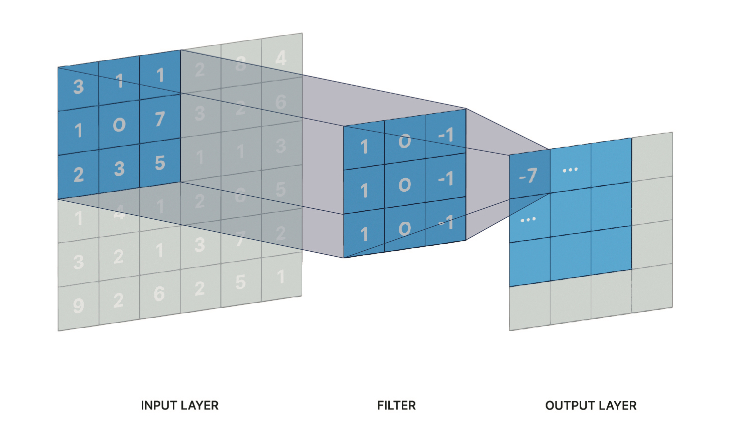
Convolution is a mathematical operation where we compute the overlap of two functions by shifting one function over the other. In order to compute the convolution at a single point, an integral is required and hence, to plot the value of the convolution over a given domain, e.g. [0.. 1], the integral has to be evaluated many times over. Although symmetric in nature, we call one function the original signal and the other 'filter'. Commonly used in digital signal processing and image manipulation, convolution has just recently been rediscovered in the field of deep learning and literally revolutionized the field. The discrete adaptation in a neural network is as follows: A convolutional layer utilizes 1..N filters of a specific size, e.g. 16x16 or 32x32. The filter 'sweeps' over the output of the previous layer, computing a weighted sum for the area that the filter momentarily hovers over. Mathematically, this corresponds to an inner product of the filter weights and the 'pixels' of the previous layer that the filter hovers over. The result is a scalar, and the output dimension of the entire layer depends on the dimension of the previous layer, the filter dimension, the 'stride' length and the padding. If the previous layer has a certain depth (think of pixels carrying color information), a 2D filter may be applied to each depth layer individually and the outputs are combined. The filter operation for a single 2D filter operating at a layer with a depth of 1 is sketched in Figure 4.

The value of a convolution is highest where areas of the previous layer and the filter weights match. Hence, the weights representing the filters can be trained to detect known patterns in the input space or the higher dimensional feature space of hidden layers. By using a large number of filters and sufficient number of layers, one can build a network that is able to recognize a person, a car, or a specific animal by training it on different input pictures that vary in size, orientation, color, lighting, and so forth. Similarly, three-dimensional filters applied to the input can be used to detect three-dimensional features (e.g. tumor cells on CAT scans or salt formation in seismic data) or sequences in regular 2D movies. Modern deep learning networks, including convolutional networks, use highly specialized layers with specific purposes. Examples are pooling layers used to reduce (spatial) dimensionality, dropout layers that literally drop connections and thereby help reduce overfitting, and batch normalization layers that help normalize the output of the previous layer to have zero mean and unit variance.

Convolutional networks have enabled pivotal advances in areas like facial recognition, medical image analysis, and self-driving cars - to name a few. In the reservoir engineering community, they create opportunities in interactive seismic interpretation, assisted well log analysis, and more.

Physics Informed Neural Network (PINN)

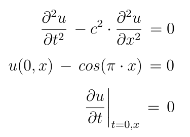
Physics informed networks have been designed primarily to solve differential equations, although we could solve other types of equations too. To those who are unfamiliar with the subject, PINNs seem to be shrouded in mystery, and hence a few facts upfront. First of all, the layer structure of a PINN is not fundamentally different from that of a MLP, specifically, the differential equation is not somehow encoded in the network. Second, a trained network will for example give us a value for u(x,t) if we present the pair (x,t) at the input. So, it is not that we present (x,t) or u(x,t) at the input and the network computes u(x,t+dt) as its output. There is no time stepping or equivalent procedure involved. For a time-dependent differential equation the network learns to map (x,t) to u(x,t) for the pairs (x,t) in a given range. In that sense, the time t is not special at all, it just adds another dimension to the input. This is quite different from traditional numerical methods that may take advantage of the unidirectional flow of time, and that difference can cause convergence issues as explained below. The main difference between a PINN and a "normal" MLP is that PINNs employ a different loss function and require extended automatic differentiation not only for the derivatives with respect to the weights, but also higher order derivatives with respect to the input variables. PINNs use unsupervised learning, that is, the loss function (or error term) is not computed by comparing the network output against an expected result (supervised learning ), but the loss function is built from the network's output alone. A short example may be best to explain how a PINN and its loss function works. Suppose we are interested in solving the wave equation with initial conditions in 1D, a classic undergraduate problem in science and engineering.

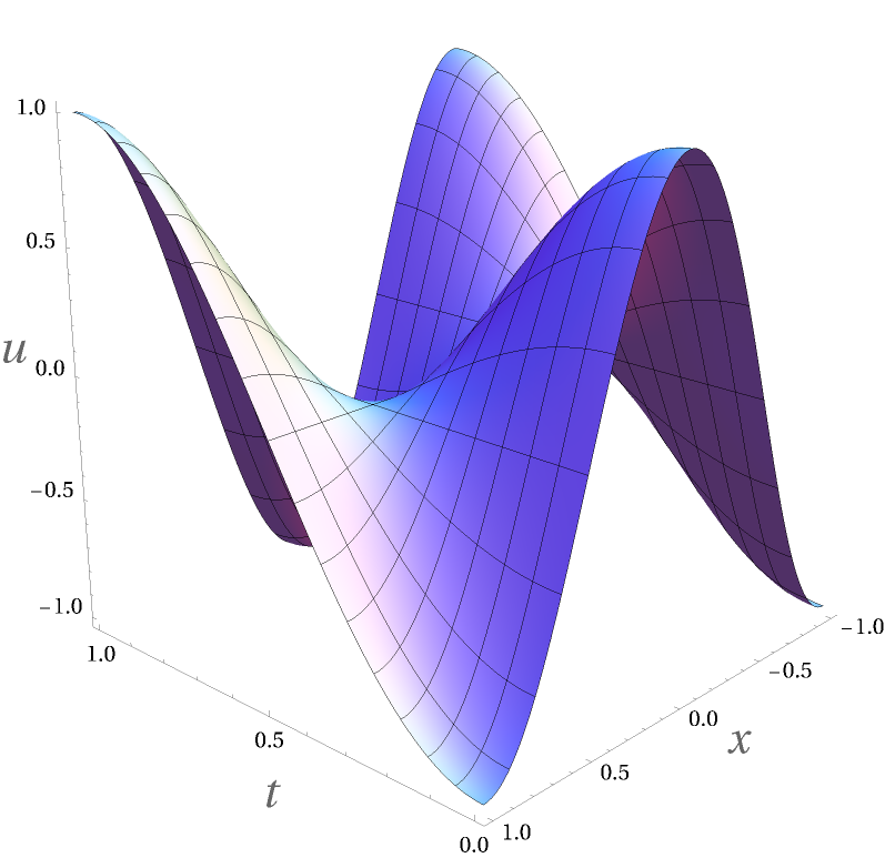
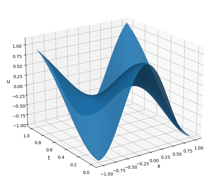
Figure 5 shows the correct solution for c=1 as computed with Wolfram Mathematica. If we follow the 'classic' approach of supervised learning to reproduce the solution with a neural network, we train the network with the analytic solution of the PDE till it has "learned" the mapping (x,t) --> u(x,t). For this particular example, this is no problem. But for many other differential equations analytic solutions are not available, especially in heterogeneous media, and we would need to build a traditional simulator to generate the training data. For a physics-informed neural network, we do not need the actual solution.

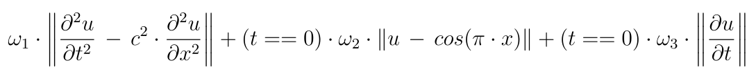
Rather than computing an error with respect to a known solution, we create a loss function based on the differential equation and the initial conditions, that is, we attempt to minimize the error represented by the equation itself. In our concrete example, the loss function would consist of three weighted parts, e.g.:

The factor (t==0) is not differentiable and in the implementation will have to be replaced by a smooth approximation. It is used for illustration here to emphasize that the last two parts enforce initial conditions while the first part enforces the PDE in the whole spatio-temporal domain.

We use automatic differentiation to compute derivatives with respect to the input variables. In other words, changes in input variables during the training are tracked and finite differencing is used to compute derivatives. This process is semi-automated in libraries like TensorFlow or PyTorch. We sometimes refer to this process as using gradient tapes because we have to record the training process to compute finite differences.

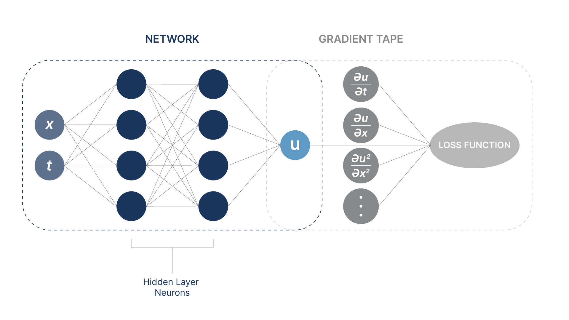
So, as we can see, we use the PDE itself to compute the loss function and hence, we do not require a known solution to train the network. That is called unsupervised learning as mentioned before. The input layer for the PINN solving the one-dimensional wave equation consists of just two neurons, with the two scalar inputs being x and t. There are several outputs needed to compute the loss function including the value of the function u, and its derivatives with respect to x and t. While the network only computes 'u', the additional machinery computes the derivatives.

The training data for the PINN is a large set of collocation points at which we perform a forward sweep and compute the loss function. The points need to be distributed dense enough in time and space to capture important features and initial and/or boundary conditions. For each collocation point or input pair (x_k,t_k) of the training set, u_k and its derivatives are computed, and the value of the loss function is determined. The gradient of the loss function with respect to the weights is then computed in the usual way, and weights are updated based on the learning parameters and optimizer used.

Figure 6 shows a PINN solution for c=1 after 1000 training epochs, using a training set with 10K samples on a 16 layer network, while Figure 7 depicts the layout of the PINN.

Limitations of PINNs

The convergence behavior of PINNs for complex physical problems is not yet fully understood, and PINNs can spectacularly fail when applied to systems exhibiting multi-scale chaotic or turbulent behavior. One problem that has been identified in the recent literature is that the training at collocation points in the spatio-temporal domain often ignores the inherent (temporal) causal structure of the problem. In other words, we may compute the PDE error and adjust weights for times t>t_0 before sufficiently reducing the error of the initial condition at t₀ This differs from traditional methods that evolve the solution over time, starting with the initial conditions. More generally speaking, the distribution of collocation points used for network evaluation and automatic differentiation during the training can be critical to the training performance and convergence rate of a PINN. We can compare this (in the spatial domain) to the problem of finding optimal points in traditional collocation methods, e.g. Gauss-Legendre integration. Recently, adaptive strategies have been developed for re-sampling the training space during the training. Such strategies have shown visible improvement in terms of training time and prediction accuracy of PINNs.

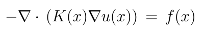
Another, more serious weakness of regular PINNs is that they 'learn' a particular differential equation using a given discretization, and have to be retrained if the equation or the underlying discretization changes. Here, we refer to the distribution and density of collocation points when we speak of the underlying discretization. This is problematic when we try to approximate parametric PDEs. For example, the steady-state elliptic PDE that describes the pressure distribution for Darcy Flow is given by:

Here, K(x) is the rock permeability or diffusion tensor that varies spatially with x. In a sense, points within the parameter space K(x) select or define points in the space of solution functions u(x) for the given PDE. A regular PINN will be trained on one particular distribution of the permeability field, and if we change K(x), we have to repeat the training. Trying to incorporate K(x) in the learning process will add one additional dimension to the input for every single discrete point x , e.g. increasing the number of input variables from three to hundreds or thousands. That makes it almost impossible to use a PINN as a surrogate model for multiple realizations where the underlying parameter space changes - as this is the case in assisted history matching for example.

Neural Operator Networks

Neural operator networks are among the latest developments in the field of deep-learning and are designed to overcome the restrictions of regular PINNs, specifically the requirement to retrain if the discretization or parametrization of a PDE changes. Their inner workings are based on or originated from kernel approximations for differential operators - hence the name. While there exist different types of neural operator networks, the most intriguing ones for solving PDEs are those which learn mappings between function spaces rather than learning a single function that maps data points between Euclidean spaces. The theory behind these networks is rather complex, and readers familiar with kernel approximations may be reminded of Green's functions and reproducing kernel Hilbert spaces. We restrict ourselves to describing the capabilities of such operator networks rather than trying to explain the theory behind it or a particular implementation. In the concrete example of the Darcy flow given above, an operator network will learn the relationship between the distribution of the parameter K(x) (rock permeability or diffusion coefficient) and the set of functions u(x) that are selected by it, based on the linear functional given by the PDE. Once that relationship has been learned, a change in the distribution of K(x) does not require us to re-train the network. Furthermore, since the operator network is trained to 'learn' a mapping between function spaces (as opposed to a mapping between data spaces), they don't need to be re-trained when the discretization changes. The latter of course assumes a certain smoothness of the operator and the parameter space. Operator networks require supervised learning that, on the downside, can become rather time intensive. The training effort however is often more than compensated by avoiding costly re-training. Among the various types of operator networks, e.g. Laplace operator networks, graph neural operator networks, or Fourier neural operator networks, the latter ones, using fast Fourier transforms have shown very promising results in the training and inference of parametric PDEs.

Forward sweeps (inference) on trained operator networks can be extremely fast. Recent research on a few selected problems demonstrated speedups of four to five orders of magnitude when comparing classic computer codes performing forward simulations with the speed of inference by a trained operator network. Even more intriguing was the ability to train the network on a coarse sample space and then conduct inference on a much finer discretization.

Potential Applications

As with other new and emerging technologies, there are high expectations for using deep learning and neural networks. While the public interest is clearly focused on generative AI (think: ChatGPT), computational scientists in the engineering community hope that neural networks can one day be used to augment finite volume and finite element-based physics simulators, avoiding complex grid generation tasks, and be able to support computing an ensemble of solutions in heterogeneous media at blistering speeds. Understanding both the opportunities and limitations is key to developing applications and directing future research. A full physics-based reservoir simulator for example, that in an automated fashion changes the course of the simulation based on conditions tested in field or well management, is actually a combination of a PDE solver with a discrete optimization machinery, trying to maximize production related quantities based on the underlying reservoir physics and a set of rules and constraints. Here, the PDE solution is just a means for driving the decision making algorithm that changes well boundary conditions (pressures and/or rates) to achieve its goals while maintaining critical physical and economical constraints. From a mathematical point of view, the time-stepping reservoir simulator solves a sequence of PDEs, each of the same type, but with evolving initial conditions and boundary values. With the current technology, we would be forced to retrain the network representing the PDE under each unique set of boundary conditions, a task taking much more time consuming then is required to take the next time step in a conventional simulator. In that sense, we think that full physics reservoir simulators will remain with us for quite some time in the future, but we also see opportunities that can materialize with the technology available today. In the following, we highlight some possible applications.

Preconditioning Equation of State (EOS) Solutions

Neural networks can be used to precondition traditional numerical algorithms with a solution estimate. This has been demonstrated to work for EOS flash computations, where neural nets have been used to predict phase envelopes for mixtures. Given that most or all energy companies have databases with fluid properties obtained via lab measurements, it is conceivable that physics informed or hybrid neural nets are being trained offline and their pre-computed weights being loaded into a simulator to assist in flash computations, especially in cases where more complex EOS computations are being considered, e.g. cubic-plus-association (cubic CPA) flash or bubble point calculations.

Computing Geomechanical Model Parameters

Recent experiments with PINNs have shown promising results in reconstructing poroelastic model parameters by solving the inverse problem associated with Biot's model equations. Due to the large number of measurement samples needed for the training, a successful application presently seems to be restricted to laboratory settings where ultrasound tomography can be applied to core samples to provide the required number of data points. Determining the coefficients from well data in the field would only make sense if wells are drilled in a very dense pattern as this is the case in shale oil and gas production.

Reinforcement Learning

Reinforcement learning is a machine learning approach where an agent learns to make decisions by assessing its environment's state, executing actions, and subsequently evaluating the cumulative rewards resulting from those actions. While the ultimate goal is to maximize cumulative rewards, an algorithm has to maintain a balance between exploring the space of possible actions by trying out new ones, and (in a greedy fashion) maximizing local rewards by sticking with proven decisions. There are different ways to accomplish this balance, e.g. slowly reducing exploration while progressing in the training, or by using stochastic methods when deciding which action to take. In any case, a reinforcement learning algorithm needs to 'remember' states of the environment, past actions, and the rewards associated with those actions. The tool for this is a discrete Q-table or a (continuous) Q-function. Q-tables are sometimes referred to as discrete Q-functions. The table's update is guided by the Bellman equation, which considers both the immediate reward from an action and a discounted future reward, factoring in the new state resulting from that action and its associated optimal (known) reward.

Neural networks (such as Deep Q networks or short: DQNs) have been successfully applied in reinforcement learning by replacing the traditional Q-table in environments with a large number of states and actions. In the reservoir community, reinforcement learning has been applied to diverse tasks such as history matching, optimal well placement, optimal well trajectory planning, and more.

Carbon Sequestration and Storage (CSS)

Modeling carbon sequestration and storage is a complex simulation task with different trapping mechanisms operating on vastly different spatio-temporal scales. The four main trapping mechanisms and their scales are:

• Structural and stratigraphic trapping (macroscopic, years)
• Residual or capillary trapping (microscopic, decades)
• Solubility trapping (microscopic, centuries)
• Mineral trapping (microscopic, millennia)

The entirety of the task is so complex that many commercial reservoir simulators can only handle certain aspects of the process, and those which can handle all are known to be rather slow. Despite the difficulties, we are excited about the use of neural operator networks specifically in that area - why? The reason for our excitement is that one doesn't need to solve all spatio-temporal scales and trapping mechanisms right from the beginning in the early phases of the global effort to sequester greenhouse gasses. The first step is to evaluate potential storage sites and simulate structural and stratigraphic trapping under uncertainty. The reader may remember that one of the obstacles to using a neural net as a replacement for a reservoir simulator in a production scenario was the frequently changing well boundary conditions and the decision-making process that resembles discrete optimization rather than a PDE solver. However, assessing the stratigraphic CO₂ trapping capacity of a formation involves very few well locations with constant injection rates maintained over long time periods. Ensemble simulations will focus on uncertainties in the geology (if the site was not used for exploration and production before) and/or optimal well placement and injection rates. Hence, there is ample opportunity to develop and experiment with solution approaches using a combination of physics-informed and operator neural networks to speed up the evaluation process, and indeed, the first results have already been reported in the field.

Closing Remarks

We have presented a short overview of the emerging technology of neural networks in the context of solving physics-based problems in the reservoir community. The presented material is far from complete and can only give a glimpse into the exciting new field. At Stone Ridge Technology, we keep a finger on the pulse of research and technology, always expanding our knowledge and looking for opportunities to improve our technical products and guide the way toward faster and more robust simulation capability.

With regard to the emerging role of neural networks in our field, we see opportunities for the use of PINNs to accelerate some of the internals of the simulator, to assist the simulator with external physical processes that couple periodically to the flow calculation and in the development of fast surrogates in simulating aspects of CO₂ sequestration and storage, using hybrid PINN and operator neural networks.